逻辑回归 #
逻辑回归(Logistic Regression) #
Logistic Regression(逻辑回归)是一种用于分类问题的统计模型,本质上是一种线性模型,通过 Sigmoid 函数将线性回归的输出映射到 (0,1) 区间,用于预测概率。分类是应用 逻辑回归(Logistic Regression) 的目的和结果, 但中间过程依旧是回归. 通过逻辑回归模型, 我们得到的计算结果是 0-1 之间的连续数字, 可以把它称为"可能性"(概率). 然后, 给这个可能性加一个阈值, 就成了分类. 例如, 可能性大于 0.5 即记为 1, 可能性小于 0.5 则记为 0。其数学公式可以表达为:
输出概率: \[ \begin{align*} &P(y=1|x) = \sigma(w^T x + b) \\ &P(y=0|x) = 1 - \sigma(w^T x + b) \\ \end{align*} \]
决策边界: \(P(y=1|x) \geq 0.5\) 时预测为1,反之预测为0。
Sigmoid 函数 #
Sigmoid 函数是一种常用的激活函数,将任意实数映射到区间 (0, 1)。 Logistic回归中,Sigmoid的输出可以帮助解释为事件发生的概率。它的数学表达式为:
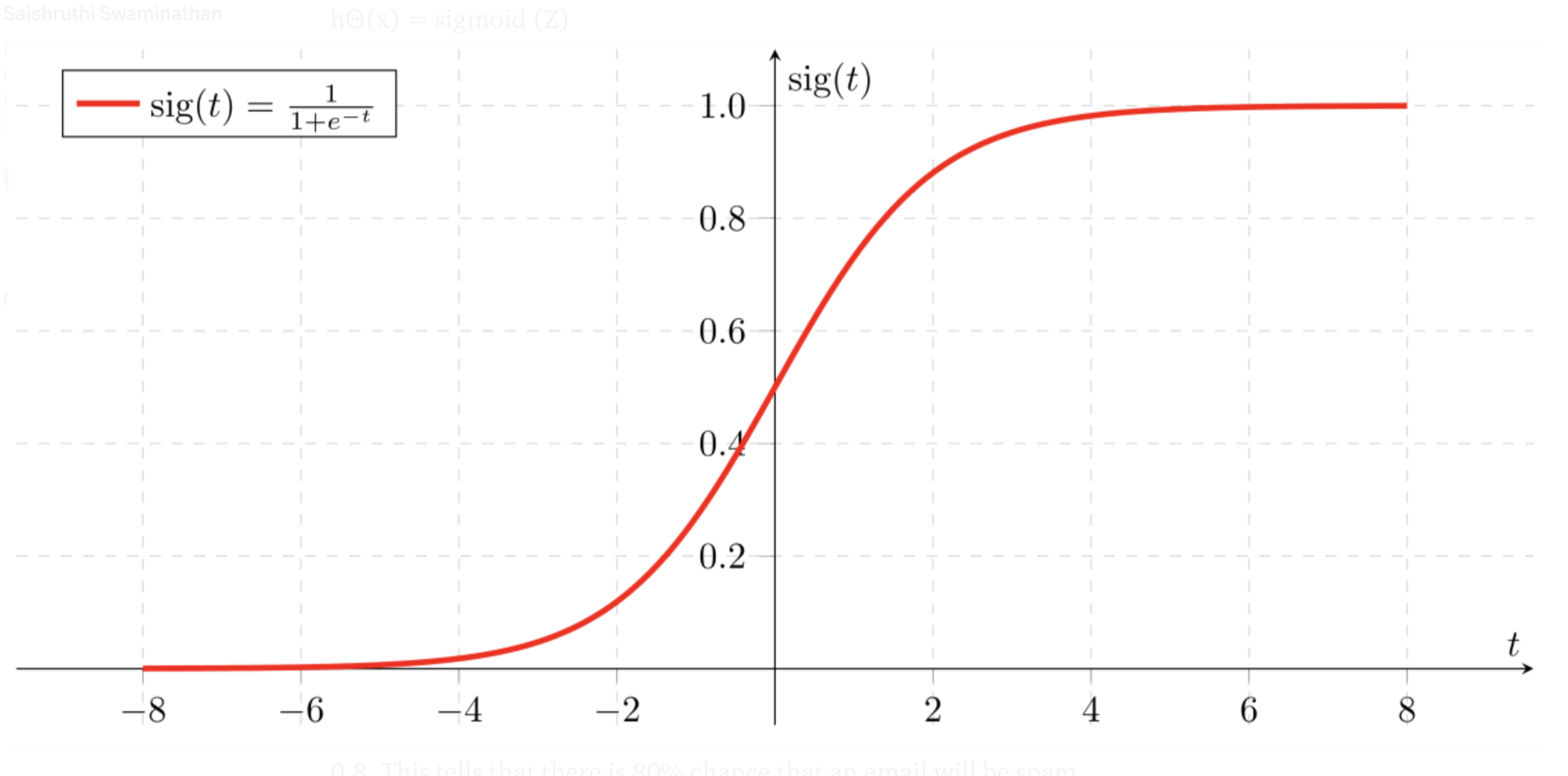
- 值域:
Sigmoid函数的输出值范围是(0, 1),这使得它特别适合用于概率预测。 - 单调递增:
Sigmoid是单调递增函数,意味着 输入值越大,输出值越接近 1。 - 中心对称:以点
(0, 0.5)为对称中心。 - 平滑性:
Sigmoid函数是光滑的,具有连续的一阶和二阶导数。
Note: 逻辑回归中,
Sigmoid函数的输出是 分类的概率,而不是分类的类别。
损失函数(Loss Function) #
Logistic 回归的训练目标是通过优化目标函数找到最优的模型参数,使模型能够对输入样本进行概率预测,并最大程度地准确分类数据,最小化训练数据的损失函数(Loss Function)。Logistic 回归的损失函数是基于 交叉熵损失(Cross-Entropy Loss) 定义的,它反映了模型预测值与实际值之间的不一致程度。
对单个样本的损失函数:Logistic 回归的损失函数采用对数似然函数的负值,针对二分类任务的每个样本: \[ \text{Loss}(y, \hat{y}) = -\left[ y \log \hat{y} + (1 - y) \log (1 - \hat{y}) \right] \]
- \(y \in \{0, 1\}\) 是实际标签。
- \(\hat{y} = P(y=1|x)\) 是模型预测的概率。
该损失函数的两种情况:
- 当 \(y = 1\) :损失为 \(-\log(\hat{y})\) ,鼓励模型将预测概率 \(\hat{y}\) 接近 1。
- 当 \(y = 0\) :损失为 \(-\log(1 - \hat{y})\) ,鼓励模型将预测概率 \(\hat{y}\) 接近 0。
总体损失函数:对整个数据集的损失函数是所有样本损失的平均值: \[ \mathcal{L}(w, b) = -\frac{1}{n} \sum_{i=1}^n \left[ y_i \log \hat{y}_i + (1 - y_i) \log (1 - \hat{y}_i) \right] \]
这里 \(\hat{y}_i = \sigma(z_i) = \frac{1}{1 + e^{-z_i}}\) ,其中 \(z_i = w^T x_i + b \) 。
梯度下降(Gradient Descent) #
Logistic Regression 使用梯度下降(Gradient Descent)优化其损失函数。在优化过程中,需要计算损失函数的梯度以更新模型参数 \(w\) , \(b\) :
损失函数对权重的梯度: \[ \frac{\partial \mathcal{L}}{\partial w} = \frac{1}{n} \sum_{i=1}^n \left[ \sigma(w^T x_i + b) - y_i \right] x_i \] 其中 \(\sigma(w^T x_i + b) - y_i\) 是预测值与真实值的误差。
损失函数对偏置的梯度: \[ \frac{\partial \mathcal{L}}{\partial b} = \frac{1}{n} \sum_{i=1}^n \left[ \sigma(w^T x_i + b) - y_i \right] \]
利用梯度更新参数: \[ w := w - \alpha \frac{\partial L}{\partial w}, \quad b := b - \alpha \frac{\partial L}{\partial b} \]
性能评估(Evaluation Metrics) #
混淆矩阵 (Confusion Matrix) #
混淆矩阵是分类模型的基本评价工具,用于总结预测结果的分类情况。对于二分类问题,矩阵包含以下四个元素:
| 预测正类 \( (\hat{y} = 1) \) | 预测负类 \((\hat{y} = 0)\) | |
|---|---|---|
| 实际正类 \((y = 1)\) | TP (True Positive) | FN (False Negative) |
| 实际负类 \((y = 0)\) | FP (False Positive) | TN (True Negative) |
- TP (True Positive): 实际为正,预测也为正。
- FN (False Negative): 实际为正,但预测为负。
- FP (False Positive): 实际为负,但预测为正。
- TN (True Negative): 实际为负,预测也为负。
准确率 (Accuracy) #
\[ \text{Accuracy} = \frac{\text{TP} + \text{TN}}{\text{TP} + \text{TN} + \text{FP} + \text{FN}} \]- 定义:模型预测正确的样本占总样本的比例。
- 优点:简单直观。
- 缺点:当类别不平衡时(正负样本比例悬殊),准确率可能误导。
精确率 (Precision) #
\[ \text{Precision} = \frac{\text{TP}}{\text{TP} + \text{FP}} \]- 描述模型预测正类的可靠性。
- 适用场景:当 FP 的代价较高时,例如垃圾邮件过滤(FP 表示误判正常邮件为垃圾邮件)。
召回率 (Recall) #
\[ \text{Recall} = \frac{\text{TP}}{\text{TP} + \text{FN}} \]- 描述模型对正类样本的捕捉能力。
- 适用场景:当 FN 的代价较高时,例如疾病检测(FN 表示漏诊病人)。
F1-Score #
\[ \text{F1-Score} = 2 \cdot \frac{\text{Precision} \cdot \text{Recall}}{\text{Precision} + \text{Recall}} \]- F1-Score 是 Precision 和 Recall 的调和平均,用于权衡两者之间的关系。
- 适用场景:当 Precision 和 Recall 同等重要时。
ROC 曲线 和 AUC (Area Under the Curve) #
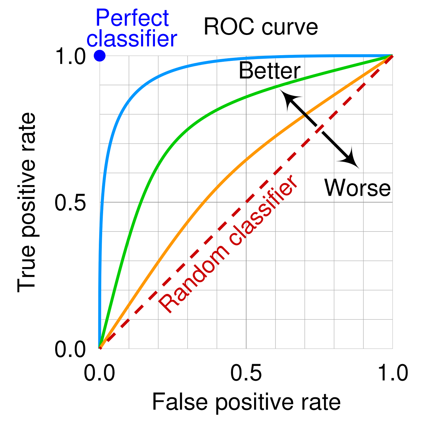
- 横轴:假正率 ( \(FPR = \frac{\text{FP}}{\text{FP} + \text{TN}}\) )。
- 纵轴:真正率 ( \(TPR = \frac{\text{TP}}{\text{TP} + \text{FN}}\) )。
- ROC 曲线展示了不同阈值下模型性能的变化。
阈值(threshold) 的变化直接影响模型的 TPR(真正例率) 和 FPR(假正例率),从而决定曲线上每个点的位置:
- 起点与终点:
- 当 阈值 = 1.0(极高阈值):所有样本都被预测为负类,
\(\text{TPR} = 0,\text{FPR} = 0\)
,即曲线起点
(0,0)。 - 当 阈值 = 0.0(极低阈值):所有样本都被预测为正类,
\(\text{TPR} = 1,\text{FPR} = 1\)
,即曲线终点
(1,1)。
- 当 阈值 = 1.0(极高阈值):所有样本都被预测为负类,
\(\text{TPR} = 0,\text{FPR} = 0\)
,即曲线起点
- 中间变化:
- 随着阈值从高到低移动,曲线从
(0,0)开始,逐渐向(1,1)延展。 - 这些点的位置和曲线的形状取决于模型在不同阈值下的 TPR 和 FPR。
- 随着阈值从高到低移动,曲线从
- 关键点:
- 特定阈值(如 0.5 或其他业务相关的值)对应的 TPR 和 FPR 可通过 ROC 图直接观察,帮助选择最佳阈值。
AUC (Area Under the Curve) #
ROC 曲线下的面积,取值范围为 [0, 1]。AUC 的意义:
- AUC = 1:完美分类器。
- AUC = 0.5:随机猜测。
- 0.5 < AUC < 1:模型有一定的区分能力。
Logistic Regression 代码实现 #
# <--- From scratch --->
import numpy as np

def sigmoid(z):
    return 1 / (1 + np.exp(-z))

def cross_entropy_loss(y, y_pred):
    """
    y: 实际标签 (0 或 1)
    y_pred: 模型预测值 (范围在 0 和 1 之间)
    返回: 平均交叉熵损失
    """
    # 防止 log(0) 导致的数值错误,添加一个小的正数 epsilon
    epsilon = 1e-15
    y_pred = np.clip(y_pred, epsilon, 1 - epsilon)  # 保证 y_pred 不会等于 0 或 1
    return -np.mean(y * np.log(y_pred) + (1 - y) * np.log(1 - y_pred))

def Logistic_Regression(X, y, lr, max_iter):
    """
    X: 特征矩阵 (n_samples x n_features)
    y: 标签向量 (n_samples,)
    lr: 学习率
    max_iter: 最大迭代次数
    返回: 训练好的权重和偏置
    """
    n_samples, n_features = X.shape  # 样本数量和特征数量
    weights = np.zeros(n_features)  # 初始化权重为 0
    bias = 0  # 初始化偏置为 0
    losses = []

    for i in range(max_iter):
        # 计算预测值
        y_pred = sigmoid(np.dot(X, weights) + bias)

        # 计算梯度
        weight_grad = (1 / n_samples) * np.dot(X.T, (y_pred - y))  # 权重的梯度
        bias_grad = (1 / n_samples) * np.sum(y_pred - y)  # 偏置的梯度

        # 计算损失并存储
        loss = cross_entropy_loss(y, y_pred)
        losses.append(loss)

        # 使用梯度下降法更新权重和偏置
        weights -= lr * weight_grad
        bias -= lr * bias_grad

    return weights, bias

def Logistic_Regression_Predict(X, weights, bias):
    # 计算预测概率
    pred_y = sigmoid(np.dot(X, weights) + bias)
    # 将概率转换为二分类标签
    return [1 if i >= 0.5 else 0 for i in pred_y]


from sklearn.datasets import make_classification
from sklearn.model_selection import train_test_split

# 生成模拟分类数据集
X, y = make_classification(n_samples=1000, n_features=10, random_state=42)
X_train, X_test, y_train, y_test = train_test_split(X, y, test_size=0.2, random_state=42)

lr = 0.1  # 学习率
max_iter = 1000  # 最大迭代次数

# 训练模型
weights, bias = Logistic_Regression(X_train, y_train, lr, max_iter)

# 使用测试集进行预测
predictions = Logistic_Regression_Predict(X_test, weights, bias)

# 打印预测结果示例
print("Predictions:", predictions[:10])
# <--- From scikit-learn --->
from sklearn.linear_model import LogisticRegression
from sklearn.model_selection import train_test_split
from sklearn.metrics import accuracy_score, confusion_matrix, classification_report
from sklearn.datasets import make_classification

X, y = make_classification(n_samples=1000, n_features=10, random_state=42)

# 数据划分
X_train, X_test, y_train, y_test = train_test_split(X, y, test_size=0.2, random_state=42)

# 模型训练
model = LogisticRegression(
    penalty='l2',       # 正则化类型:'l1', 'l2', 'elasticnet', 或 'none'(默认 'l2')
    C=1.0,              # 正则化强度的倒数,值越小正则化越强,默认为 1.0
    solver='lbfgs',     # 优化算法:如 'lbfgs', 'liblinear', 'sag', 'saga' 等
    max_iter=100,       # 最大迭代次数,防止迭代过多导致训练时间过长
    random_state=42     # 随机种子,保证结果可复现
)
model.fit(X_train, y_train)

# 预测
y_pred = model.predict(X_test)

# 评价指标
accuracy = accuracy_score(y_test, y_pred)
conf_matrix = confusion_matrix(y_test, y_pred)
report = classification_report(y_test, y_pred)

print(f"Accuracy: {accuracy}")
print(f"Confusion Matrix:\n{conf_matrix}")
print(f"Classification Report:\n{report}")