
Binary Logistic Regression is one of the most simple and commonly used Machine Learning algorithms for two-class classification. It is easy to implement and can be used as the baseline for any binary classification problem. Its basic fundamental concepts are also constructive in deep learning. Logistic regression describes and estimates the relationship between one dependent binary variable and independent variables.
“分类"是应用 逻辑回归(Logistic Regression) 的目的和结果, 但中间过程依旧是"回归”. 通过逻辑回归模型, 我们得到的计算结果是0-1之间的连续数字, 可以把它称为"可能性"(概率). 然后, 给这个可能性加一个阈值, 就成了分类. 例如, 可能性大于 0.5 即记为 1, 可能性小于 0.5 则记为 0.
The classification problem is just like the regression problem, except that the values we now want to predict take on only a small number of discrete values. For now, we will focus on the binary classification problem in which \(y\) can take on only two values, 0 and 1. (Most of what we say here will also generalize to the multiple-class case.)
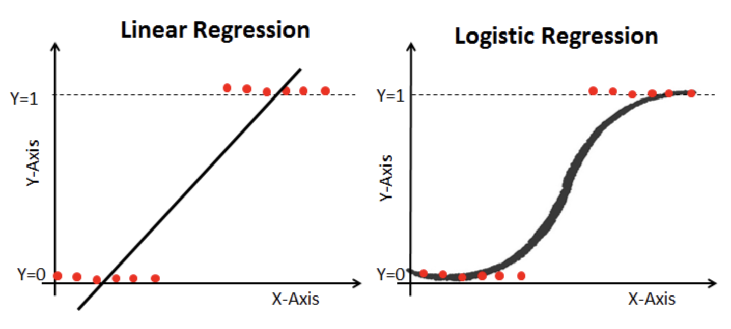
\[ log\frac{p}{1-p} = \beta_{0} + \beta_{1}x_{1} + \beta_{2}x_{2} + \beta_{3}x_{3} + \cdot\cdot\cdot + \beta_{n}x_{n} = \beta^{T}x \\ \] \[ \begin{align*} P(y = 1) &= p = \frac{e^{\beta^{T}x}}{1+e^{\beta^{T}x}} \\ P(y = 0) &= 1 - p = \frac{1}{1+e^{\beta^{T}x}} \end{align*} \]We could approach the classification problem ignoring the fact that \(y\) is discrete-valued, and use our old linear regression algorithm to try to predict \(y\) given \(x\) . However, it is easy to construct examples where this method performs very poorly. Intuitively, it also doesn’t make sense for \(h_{\theta}(x)\) to take values larger than 1 or smaller than 0 when we know that \(y \in {0, 1}\) . To fix this, let’s change the form for our hypotheses \(h_{\theta}(x)\) to satisfy \(0 \leq h_{\theta}(x) \leq 1\) This is accomplished by plugging \(\theta^{T}x\) into the Logistic Function. Our new form uses the “Sigmoid Function,” also called the “Logistic Function”:
\[ f(x) = \frac{1}{1+e^{-(x)}} \\ \]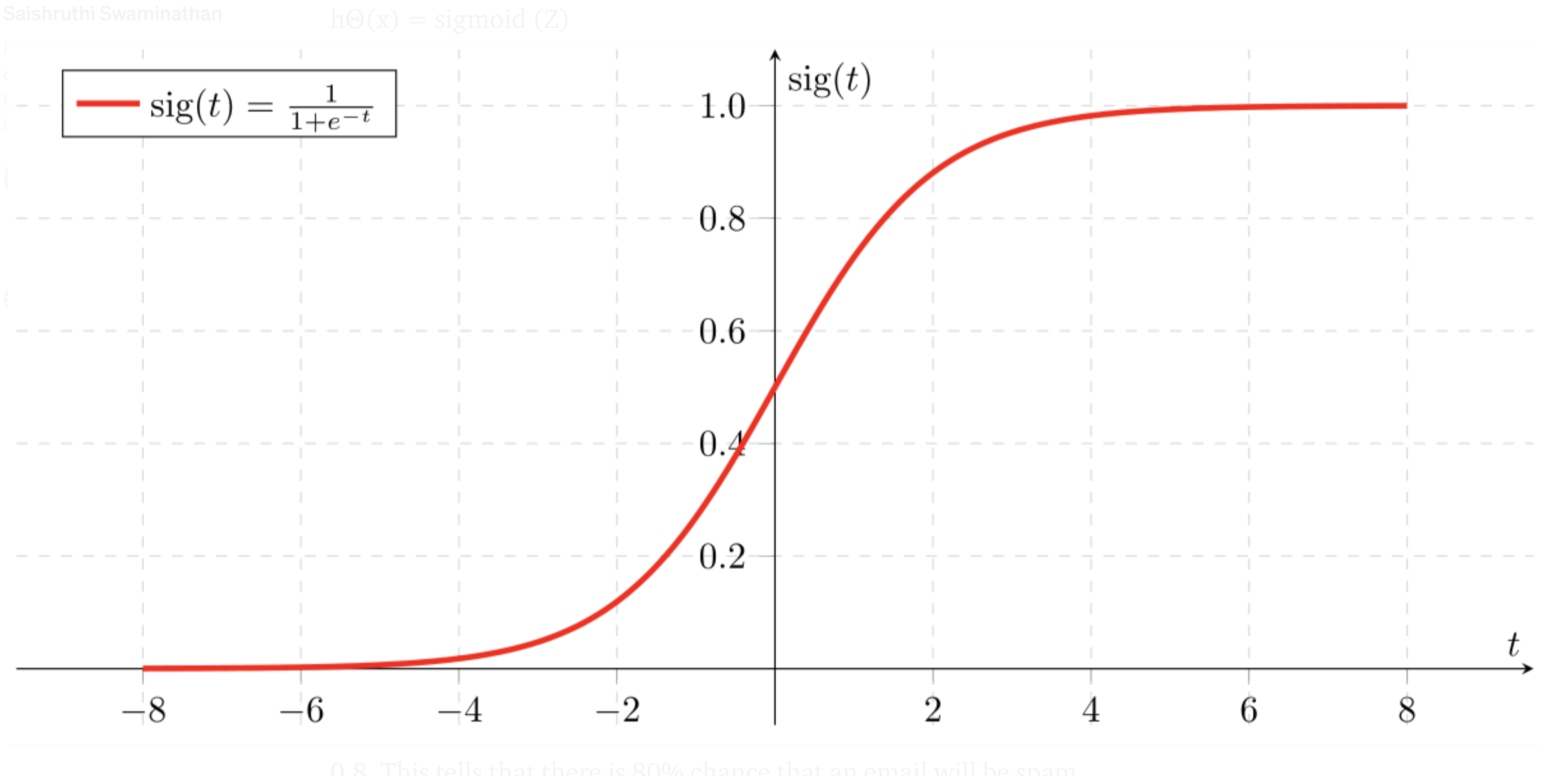
Logistic Regression #
First we need to define a Probability Mass Function:
\[ \begin{align*} &\ \ \ \ \ \ \ \ \ \ P(Y=1|X=x) = \frac{e^{\beta^{T}x}}{1+e^{\beta^{T}x}} \\ &\ \ \ \ \ \ \ \ \ \ P(Y=0|X=x) = 1 - \frac{e^{\beta^{T}x}}{1+e^{\beta^{T}x}} = \frac{1}{1+e^{\beta^{T}x}} \\ &\Rightarrow \ \ \ \ P(Y \ |X=x_{i}) = (\frac{e^{\beta^{T}x_{i}}}{1+e^{\beta^{T}x_{i}}})^{y_{i}} (\frac{1}{1+e^{\beta^{T}x_{i}}})^{1-y_{i}} \\ \end{align*} \]Naturally, we want to maximize the right-hand-side of the above statement. We will use Maximun Likelihood Estimation(MLE) to find \(\beta\) :
\[ \hat{\beta}_{MLE}= \arg\max_{\beta} L(\beta) \\ \] \[ L(\beta) = \prod_{i=1}^n P(Y=y_{i} |x_{i}) = \prod_{i=1}^n (\frac{e^{\beta^{T}x_{i}}}{1+e^{\beta^{T}x_{i}}})^{y_{i}} (\frac{1}{1+e^{\beta^{T}x_{i}}})^{1-y_{i}} \\ \] \[ \begin{align*} l(\beta) = log\ L(\beta) &= \sum_{i=1}^n y_{i}\left[\beta^{T}x_{i} - log(1+e^{\beta^{T}x_{i}})] + (1-y_{i})[-log(1+e^{\beta^{T}x_{i}})\right] \\ &=\sum_{i=1}^n y_{i}\beta^{T}x_{i}- log(1+e^{\beta^{T}x_{i}}) \\ \end{align*} \]Newton‐Raphson Method for Binary Logistic Regression #
Newton’s Method is an iterative equation solver: it is an algorithm to find the roots of a convex function. Equivalently, the method solves for root of the derivative of the convex function. The idea behind this method is ro use a quadratic approximate of the convex function and solve for its minimum at each step. For a convex function \(f(x)\) , the step taken in each iteration is \(-(\nabla^{2}f(x))^{-1}\nabla f(x)\) . while \(\lVert\nabla f(\beta)\rVert > \varepsilon\) :
\[ \beta^{new} = \beta^{old}-(\nabla^{2}f(x))^{-1}\nabla f(x) \\ \]Where \(\nabla f(x)\) is the Gradient of \(f(x)\) and \(\nabla^{2} f(x)\) is the Hessian Matrix of \(f(x)\) .
\[ \begin{align*} \nabla f(x) = \frac{\partial l}{\partial \beta} &= \sum_{i=1}^n y_{i}x_{i}- (\frac{e^{\beta^{T}x_{i}}}{1+e^{\beta^{T}x_{i}}})\cdot x_{i}^{T} \\ &= \sum_{i=1}^n (y_{i}- \underbrace{\frac{e^{\beta^{T}x_{i}}}{1+e^{\beta^{T}x_{i}}}}_{p_{i}})\cdot x_{i}^{T} = X(y-p) \\ \end{align*} \] \[ \nabla^{2}f(x) = \frac{\partial^{2} l}{\partial \beta \partial \beta^{T}} = \sum_{i=1}^n - \underbrace{\frac{e^{\beta^{T}x_{i}}}{1+e^{\beta^{T}x_{i}}}}_{p_{i}}\cdot \underbrace{\frac{1}{1+e^{\beta^{T}x_{i}}}}_{1-p_{i}}x_{i} \cdot x_{i}^{T} = -XWX^{T} \\ \]Where \(W\) is a diagonal \((n,n)\) matrix with the \(i^{th}\) diagonal element defined as
\[ W = \begin{bmatrix} p_{i}(1-p_{i}) & & \\ & \ddots & & \\ & & & \\ \end{bmatrix}_{\ n x n} \\ \]The Newton‐Raphson algorithm can now be expressed as:
\[ \begin{align*} \beta^{new} &= \beta^{old}-(\nabla^{2}f(x))^{-1}\nabla f(x) \\ &= \beta^{old}+ (XWX^{T})^{-1}X(y-p) \\ &= \beta^{old}+ (XWX^{T})^{-1}[XWX^{T}\beta^{t}+ X(y-p)] \\ &= \beta^{old}+ (XWX^{T})^{-1}XWZ \\ \end{align*} \]Where \(Z\) can be expressed as: \(Z = X^{T}\beta^{t}+ W^{-1}(y-p) \) . This algorithm is also known as Iteratively Reweighted Least Squares(IRLS).
\[ \beta^{t+1} = \arg\min_{\beta}(Z - X\beta)^{T}W(Z-X\beta) \\ \]Other types of Logistic Regression #
Multinomial Logistic Regression #
Three or more categories without ordering. Example: Predicting which food is preferred more (Veg, Non-Veg, Vegan).
Ordinal Logistic Regression #
Three or more categories with ordering. Example: Movie rating from 1 to 5.
References #
[1] K, D. (2021, April 8). Logistic Regression in Python using Scikit-learn. Medium. https://heartbeat.fritz.ai/logistic-regression-in-python-using-scikit-learn-d34e882eebb1.
[2] Li, S. (2019, February 27). Building A Logistic Regression in Python, Step by Step. Medium. https://towardsdatascience.com/building-a-logistic-regression-in-python-step-by-step-becd4d56c9c8.
[3] Christian. (2020, September 17). Plotting the decision boundary of a logistic regression model. https://scipython.com/blog/plotting-the-decision-boundary-of-a-logistic-regression-model/.